阅读量： 672

Chapter 7

7.4 Mean Field Theory

the Ising model Hamiltonian,

\hat{H}=-J \sum_{\langle i j\rangle} \sigma_{i} \sigma_{j}-H \sum_{i} \sigma_{i}

$\text { We will write }\left\langle\sigma_{i}\right\rangle \equiv m$ , then we have

\begin{aligned} \sigma_{i} \sigma_{j} &=\left(m+\delta \sigma_{i}\right)\left(m+\delta \sigma_{j}\right) \\ &=m^{2}+m\left(\delta \sigma_{i}+\delta \sigma_{j}\right)+\delta \sigma_{i} \delta \sigma_{j} \\ &=-m^{2}+m\left(\sigma_{i}+\sigma_{j}\right)+\delta \sigma_{i} \delta \sigma_{j} . \end{aligned}

neglect the last term on RHS, substitute it in Hamiltonian,

\hat{H}_{\mathrm{MF}}=\frac{1}{2} N z J m^{2}-(H+z J m) \sum_{i} \sigma_{i}

define

H_{\mathrm{eff}}=H+z J m

which indicates the effective “mean field”.

We find the partition function of the canonical ensemble and the free energy that

\begin{aligned} Z &=\sum_{state} e^{-\beta \hat{H}} \\ &=e^{-\frac{\beta}{2} N z J m^{2}} \cdot(2 \cosh \beta(H+2 J m))^{N} \end{aligned}\\ \begin{aligned} F &=-K_{B} T \ln Z \\ &=\frac{1}{2} N z J m^{2}-N K_{B} T \ln 2 \cosh \beta(H+z J m) \end{aligned}

adimensionalize the free energy

f(m, h, \theta)=\frac{1}{2} m^{2}-\theta \ln \left(e^{(m+h) / \theta}+e^{-(m+h) / \theta}\right) .

We know that we have to minimize the free energy at equilibrium under constant volume and constant temperature, so we can get the mean field equation by differentiate $f$

m=\tanh \left(\frac{m+h}{\theta}\right)

discussion:

(i) $h=0$

m=\tanh \left(\frac{m}{\theta}\right)

if $\theta\ge 1$ , one solution $m=0$ . If $\theta <1$ , three solutions and they are symmetric. It means spontaneous magnetization occurs at the point.

\theta_C=1

is the mean field transition temperature, and its a second-order transition.

Also we find for $|\theta-1| \ll 1$ ,

m(\theta, h=0)=\pm \sqrt{3}(1-\theta)_{+}^{1 / 2}

the exponent $\beta$ equals 1/2.

now we compute the heat capacity. $\text { When } \theta \geqslant 1, m=0, \quad f=-\theta \ln 2 \quad c_{v}=0 \text { . }$

when $\theta<1$ ,

f=\frac{m^{2}}{2}-\theta\ln\left(2 \cosh \frac{m}{\theta}\right)

c_{V}=-\theta \frac{\partial^{2} f}{\partial \theta^{2}}=\frac{1}{\theta} \cdot \frac{m^{2}(\theta)-m^{4}(\theta)}{\theta-1+m^{2}(\theta)}

the calculation is not complex.

$\text { Let } \theta \rightarrow 1 \text { and use } m^{2} \simeq 3 \theta^{2}\left(1-\theta^{2}\right)$ , we can obtain $c_V\rightarrow \frac32$

(ii)sets $\frac{\partial f}{\partial m}=0$ and $\frac{\partial^{2} f}{\partial m^{2}}=0$ simultaneously, resulting in

h^{*}(\theta)=\sqrt{1-\theta}-\frac{\theta}{2} \ln \left(\frac{1+\sqrt{1-\theta}}{1-\sqrt{1-\theta}}\right) .

$\text { The solutions lie at } h=\pm h^{*}(\theta) . \text { For } \theta<\theta_{\mathrm{c}}=1 \text { and } h \in\left[-h^{*}(\theta),+h^{*}(\theta)\right]$ , there are three solutions to the mean field equation

Setting $\frac{\partial f}{\partial m}=0$ , we obtain

\frac{1}{3} m^{3}+(\theta-1) \cdot m-h=0 \text { . }

still assumed $h \ll|\theta-1| \ll 1$ ,

if $\theta >1$ we have

m=h /(\theta-1)

and we can obtain the Curie-Weiss law, which shows the critical exponent $\gamma=1$

\chi(\theta)=\frac{\partial m}{\partial h}=\frac{1}{\theta-1} \propto|\theta-1|^{-\gamma}

if $\theta <1$ , the solution above becomes a maxima, and the minima is

m(\theta, h)=\sqrt{3}(1-\theta)+\frac{h}{2(1-\theta)}

the critical exponent $\gamma$ is also 1.

if $\theta=1$ ,

m\left(\theta=\theta_{\mathrm{c}}, h\right)=(3 h)^{1 / 3} \propto h^{1 / \delta}

In fact, it turns out that the mean field exponents are exact provided d > du, where du is the upper critical dimension of the theory. For the Ising model, du = 4, and above four dimensions (which is of course unphysical) the mean field exponents are in fact exact.

dynamics

7.5 Variational Density Matrix Method

Suppose we are given a Hamiltonian $\hat{H}$ . From this we construct the free energy, $F$ :

\begin{aligned} F &=E-T S \\ &=\operatorname{Tr}(\varrho \hat{H})+k_{\mathrm{B}} T \operatorname{Tr}(\varrho \ln \varrho) \end{aligned}

Let us assume that ̺ is diagonal in the basis of eigenstates of ˆH , i.e.

\varrho=\sum_{\gamma} P_{\gamma}|\gamma\rangle\langle\gamma|

use it to calculate Ising model

\hat{H}=-\sum_{i<j} J_{i j} \sigma_{i} \sigma_{j}-H \sum_{i} \sigma_{i}

We now write a trial density matrix which is a product over contributions from independent single sites:

\varrho_{N}\left(\sigma_{1}, \sigma_{2}, \ldots\right)=\prod_{i} \varrho\left(\sigma_{i}\right)

where

\varrho(\sigma)=\left(\frac{1+m}{2}\right) \delta_{\sigma, 1}+\left(\frac{1-m}{2}\right) \delta_{\sigma,-1} .

adopt another notation

\varrho=\left(\begin{array}{cc} \frac{1+m}{2} & 0 \\ 0 & \frac{1-m}{2} \end{array}\right)\\ \varrho_{N}=\varrho \otimes \varrho \otimes \cdots \otimes \varrho

so that we can use $Tr(A\otimes B)=Tr(A)Tr(B)$ to evaluate F and S:

\begin{aligned} E &=\operatorname{Tr}\left(\varrho_{N} \hat{H}\right)=-\sum_{i<j} J_{i j} m^{2}-H \sum_{i} m \\ &#038;=-\frac{1}{2} N \hat{J}(0) m^{2}-N H m \end{aligned} \\ \begin{aligned} S &#038;=-k_{\mathrm{B}} \operatorname{Tr}\left(\varrho_{N} \ln \varrho_{N}\right)=-N k_{\mathrm{B}} \operatorname{Tr}(\varrho \ln \varrho) \\ &#038;=-N k_{\mathrm{B}}\left\{\left(\frac{1+m}{2}\right) \ln \left(\frac{1+m}{2}\right)+\left(\frac{1-m}{2}\right) \ln \left(\frac{1-m}{2}\right)\right\} . \end{aligned}

and we can obtain the dimensionless free energy per site

f(m, h, \theta)=-\frac{1}{2} m^{2}-h m+\theta\left\{\left(\frac{1+m}{2}\right) \ln \left(\frac{1+m}{2}\right)+\left(\frac{1-m}{2}\right) \ln \left(\frac{1-m}{2}\right)\right\}

We extremize $f(m)$ by setting

\begin{array}{c} \frac{\partial f}{\partial m}=0=-m-h+\frac{\theta}{2} \ln \left(\frac{1+m}{1-m}\right) . \\ m=\tanh \left(\frac{m+h}{\theta}\right) \end{array}

which is the same as the result of mean field theory. The discussion next is quite the same. In 7.10 we will see the equivalence of the two methods.

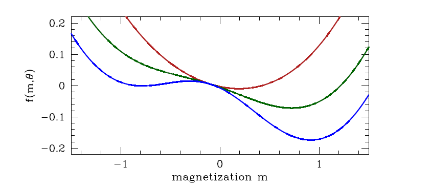
7.6 Landau Theory of Phase Transitions

based on expansion of the free energy of a thermodynamic system in terms of an order parameter

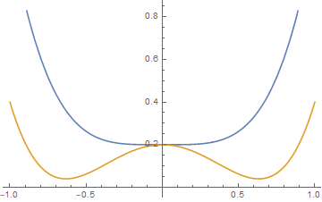
(1) quartic free energy

f(m, h, \theta)=f_{0}+\frac{1}{2} a m^{2}+\frac{1}{4} b m^{4}-h m

(i) h=0

symmetric

\frac{\partial f}{\partial m}=0=a m+b m^{3}

unique temperature θc where a(θc) = 0

\begin{array}{l} \theta<\theta_{\mathrm{c}} \quad: \quad f(\theta)=f_{0}-\frac{a^{2}}{4 b} \\ \theta>\theta_{\mathrm{c}} \quad: \quad f(\theta)=f_{0} \end{array}

c\left(\theta_{\mathrm{c}}^{+}\right)-c\left(\theta_{\mathrm{c}}^{-}\right)=-\left.\theta_{\mathrm{c}} \frac{\partial^{2}}{\partial \theta^{2}}\right|_{\theta=\theta_{\mathrm{c}}}\left(\frac{a^{2}}{4 b}\right)=-\frac{\theta_{\mathrm{c}}\left[a^{\prime}\left(\theta_{\mathrm{c}}\right)\right]^{2}}{2 b\left(\theta_{\mathrm{c}}\right)}

$\theta_C$ 二阶相变点，比热突变

1h0

(ii)h≠0

asymmetric

b m^{3}+a m-h=0 .

$f^{\prime \prime}(m)=0$ as well as $f^{\prime}(m)=0$ we can obtain

a^{*}(h)=-\frac{3}{2^{2 / 3}} b^{1 / 3}|h|^{2 / 3}

$a<a^{*}(h)$ , then there will be three real solutions to the mean field equation $f^{\prime}(m)=0$ , one of which is a global minimum (the one for which $m \cdot h>0$ ).

For $a>a^{*}(h)$ one minima disappear and there is only a single global minimum

一阶相变

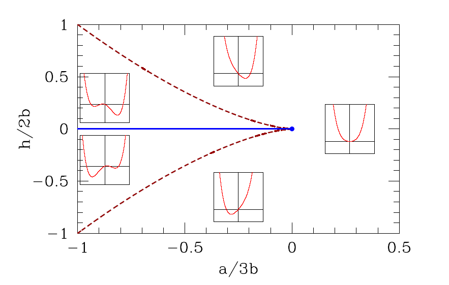
(2) cubic terms

f=f_{0}+\frac{1}{2} a m^{2}-\frac{1}{3} y m^{3}+\frac{1}{4} b m^{4}\\ \frac{\partial f}{\partial m}=0=a m-y m^{2}+b m^{3}

we can obtain

\begin{aligned} a>\frac{y^{2}}{4 b} &: 1 \text { real root } m=0 \\ \frac{y^{2}}{4 b}>a>\frac{2 y^{2}}{9 b} &: 3 \text { real roots; minimum at } m=0 \\ \frac{2 y^{2}}{9 b}>a &: 3 \text { real roots; minimum at } m=\frac{y}{2 b}+\sqrt{\left(\frac{y}{2 b}\right)^{2}-\frac{a}{b}} \end{aligned}

thus $y^{2}=\frac{9}{2} a b$ denotes a line of first order transitions

if we impose some dynamics on the system, adimensionalize the free energy

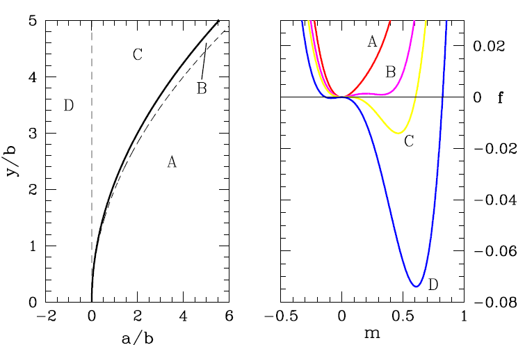
m \equiv \frac{y}{b} \cdot u \quad, \quad a \equiv \frac{y^{2}}{b} \cdot r \quad, \quad t \equiv \frac{b}{\Gamma y^{2}} \cdot s \\ \varphi(u)=\frac{1}{2} r u^{2}-\frac{1}{3} u^{3}+\frac{1}{4} u^{4} .

3-2

(3)Sixth order Landau theory : tricritical point

f=f_{0}+\frac{1}{2} a m^{2}+\frac{1}{4} b m^{4}+\frac{1}{6} c m^{6}\\ \frac{\partial f}{\partial m}=0=m\left(a+b m^{2}+c m^{4}\right)

(i) $\text { If } a>0 \text { and } b>0$ , $\text { a unique minimum at } m=0 \text { . }$

(ii) $\text { For } a<0$ , One of the solutions is $m=0$ . The other two are

m=\pm \sqrt{-\frac{b}{2 c}+\sqrt{\left(\frac{b}{2 c}\right)^{2}-\frac{a}{c}}}

(iii) $a>0 \text { and } b<0$

\begin{aligned} &\begin{aligned} b>-2 \sqrt{a c} &: & 1 \text { real root } m=0 \\ -2 \sqrt{a c}>b>-\frac{4}{\sqrt{3}} \sqrt{a c} &: & 5 \text { real roots; minimum at } m=0 \end{aligned}\\ &-\frac{4}{\sqrt{3}} \sqrt{a c}>b \quad: \quad 5 \text { real roots; minima at } m=\pm \sqrt{-\frac{b}{2 c}+\sqrt{\left(\frac{b}{2 c}\right)^{2}-\frac{a}{c}}} \end{aligned}

The point (a, b) = (0, 0), which lies at the confluence of a first order line and a second order line, is known as a tricritical point.

dynamics

m \equiv \sqrt{\frac{|b|}{c}} \cdot u \quad, \quad a \equiv \frac{b^{2}}{c} \cdot r \quad, \quad t \equiv \frac{c}{\Gamma b^{2}} \cdot s .\\ \varphi(u)=\frac{1}{2} r u^{2} \pm \frac{1}{4} u^{4}+\frac{1}{6} u^{6} .

7.11.3 Canted quantum antiferromagnet

Consider the following model for quantum $S=\frac{1}{2}$ spins:

\hat{H}=\sum_{\langle i j\rangle}\left[-J\left(\sigma_{i}^{x} \sigma_{j}^{x}+\sigma_{i}^{y} \sigma_{j}^{y}\right)+\Delta \sigma_{i}^{z} \sigma_{j}^{z}\right]+\frac{1}{4} K \sum_{\langle i j k l\rangle} \sigma_{i}^{z} \sigma_{j}^{z} \sigma_{k}^{z} \sigma_{l}^{z}

we include a parameter α which describes the canting angle that the spins on these sublattices make with respect to the ˆx-axis.

so the variational density matrix of each site is

\begin{array}{l} \varrho_{\mathrm{A}}=\frac{1}{2}+\frac{1}{2} m\left(\sin \alpha \sigma^{x}+\cos \alpha \sigma^{z}\right) \\ \varrho_{\mathrm{B}}=\frac{1}{2}+\frac{1}{2} m\left(\sin \alpha \sigma^{x}-\cos \alpha \sigma^{z}\right) \end{array}

Finally, the eigenvalues of $\varrho_{\mathrm{A}, \mathrm{B}}$ are still $\lambda_{\pm}=\frac{1}{2}(1 \pm m)$ , hence

\begin{aligned} s(m) & \equiv-\operatorname{Tr}\left(\varrho_{\mathrm{A}} \ln \varrho_{\mathrm{A}}\right)=-\operatorname{Tr}\left(\varrho_{\mathrm{B}} \ln \varrho_{\mathrm{B}}\right) \\ &=-\left[\frac{1+m}{2} \ln \left(\frac{1+m}{2}\right)+\frac{1-m}{2} \ln \left(\frac{1-m}{2}\right)\right] . \end{aligned}

the calculation is similar to the 7.5, we can obtain the free energy and adimensionalize it

\begin{aligned} F &=\operatorname{Tr}(\varrho \hat{H})+k_{\mathrm{B}} T \operatorname{Tr}(\varrho \ln \varrho) \\ &=-2 N\left(J \sin ^{2} \alpha+\Delta \cos ^{2} \alpha\right) m^{2}+\frac{1}{4} N K m^{4} \cos ^{4} \alpha-N k_{\mathrm{B}} T s(m) \end{aligned}\\ f(m, \alpha)=-\frac{1}{2} m^{2}+\frac{1}{2}(1-\delta) m^{2} \cos ^{2} \alpha+\frac{1}{4} \kappa m^{4} \cos ^{4} \alpha-\theta s(m)

in it, $f \equiv F / 4 N J,\delta \equiv \Delta / J, \kappa \equiv K / 4 J, \text { and } \theta \equiv k_{\mathrm{B}} T / 4 J$

similarly to find its minima, we have

\begin{array}{l} \frac{\partial f}{\partial m}=0=-m+(1-\delta) m \cos ^{2} \alpha+\kappa m^{3} \cos ^{4} \alpha+\frac{1}{2} \theta \ln \left(\frac{1+m}{1-m}\right) \\ \frac{\partial f}{\partial \alpha}=0=\left(1-\delta+\kappa m^{2} \cos ^{2} \alpha\right) m^{2} \sin \alpha \cos \alpha \end{array}

and we can obtain

\cos ^{2} \alpha=\left\{\begin{array}{ll} 0 & \text { if } \delta<1 \\ (\delta-1) / \kappa m^{2} &#038; \text { if } 1 \leq \delta \leq 1+\kappa m^{2} \\ 1 &#038; \text { if } \delta \geq 1+\kappa m^{2} \end{array}\right.

discussion:

(i) $\delta<1$ , $\cos \alpha=0$ , $m=\tanh (m / \theta)$ , so A and B have no difference in angles. The solution is the same as discussed above.

(ii) $1<\delta<1+\kappa m^{2}$ , we have canting with an angle

\alpha=\alpha^{*}(m)=\cos ^{-1} \sqrt{\frac{\delta-1}{\kappa m^{2}}}

$\text { we can also obtain the relation } m=\tanh (m / \theta)$ , and the boundary is

\theta_{0}=\frac{m_{0}}{\tanh ^{-1}\left(m_{0}\right)}<1 \quad ; \quad m_{0}=\sqrt{\frac{\delta-1}{\kappa}}

(iii) $\theta>\theta_{0} \text { , we have } \delta>1+\kappa m^{2} \text { , and we must take } \cos ^{2} \alpha=1 \text { . }$

\delta m-\kappa m^{3}=\frac{\theta}{2} \ln \left(\frac{1+m}{1-m}\right)

through this equation we can obtain m.

A brief summary of Chapter 7: MEAN FIELD THEORY OF PHASE TRANSITIONS

A brief summary of Chapter 7: MEAN FIELD THEORY OF PHASE TRANSITIONS

Chapter 7

7.4 Mean Field Theory

7.5 Variational Density Matrix Method

7.6 Landau Theory of Phase Transitions

(1) quartic free energy

(2) cubic terms

(3)Sixth order Landau theory : tricritical point

7.11.3 Canted quantum antiferromagnet

留下回复取消回复

A brief summary of Chapter 7: MEAN FIELD THEORY OF PHASE TRANSITIONS

Chapter 7

7.4 Mean Field Theory

7.5 Variational Density Matrix Method

7.6 Landau Theory of Phase Transitions

(1) quartic free energy

(2) cubic terms

(3)Sixth order Landau theory : tricritical point

7.11.3 Canted quantum antiferromagnet

留下回复 取消回复

留下回复取消回复